Saturday, December 10, 2011

Creating Degenerated dimension

Degenerate Dimensions
In a data warehouse, a degenerate dimension is a dimension which is derived from the fact table and doesn't have its own dimension table. Degenerate dimensions are often used when a fact table's grain represents transactional level data and one wishes to maintain system specific identifiers such as order numbers, invoice numbers and the like without forcing their inclusion in their own dimension. The decision to use degenerate dimensions is often based on the desire to provide a direct reference back to a transactional system without the overhead of maintaining a separate dimension table.

Once a cube is created, we can add degenerate dimension to the cube.
Below are the steps to create Degenerate Dimension:

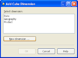
1. Click on Add Cube Dimension icon in Dimension Usage tab as shown below. It will open Add Cube Dimension dialogue box.
2. Click on New dimension… button in Add Cube Dimension dialogue box.


3. It will open Dimension Wizard. Click on Next to continue…
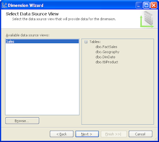
4. Select required data source view and click on Next to continue…


5. Select Standard dimension option and click on Next to continue…
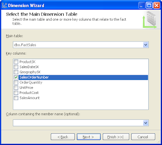
6. Select Main Dimension table and Key columns. Click on Next to continue…  
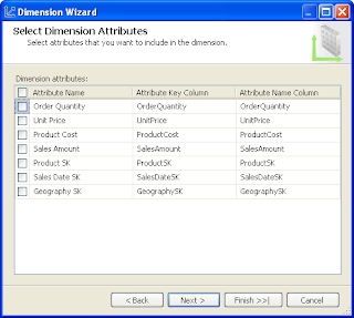
7. Select Dimension Attributes. Click on Next to continue…  


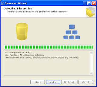
8. Click on Next to continue…  


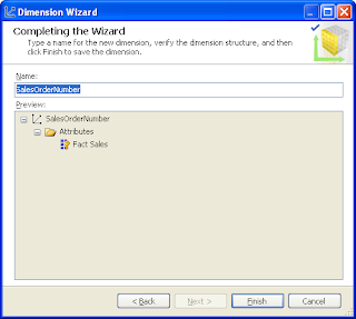
9. Now we are at Completing the Wizard. Give proper dimension name click Finish to complete.


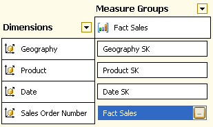
10. Newly created dimension is now available in Dimension Usage tab. At the intersection of Fact Sales measure group and the Sales Order Number dimension, click the ellipsis button (…) in the Item Description cell to review the fact relationship properties.   


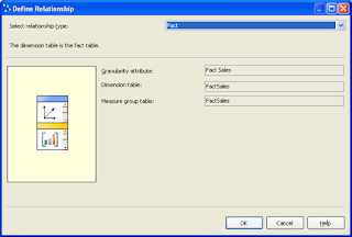
The Define Relationship dialog box opens. Notice that you cannot configure any of the properties. The Selected relationship type should be Fact.

The following image shows the fact relationship properties in the Define Relationship dialog box


Tuesday, November 1, 2011

Key Performance Indicators (KPIs) using Analysis Services

In business terminology, a KPI is a quantifiable measurement for gauging business success. In Analysis Services, a KPI is a collection of calculations that are associated with a measure group in a cube that are used to evaluate business success. Typically, these calculations are a combination of Multidimensional Expressions (MDX) expressions or calculated members. KPIs also have additional metadata that provides information about how client applications should display the results of the KPI's calculations

Common KPI Terms:
  • Goal - An MDX numeric expression or a calculation that returns the target value of the KPI.
  • Value - An MDX numeric expression that returns the actual value of the KPI.
  • Status - An MDX expression that represents the state of the KPI at a specified point in time. The status MDX expression should return a normalized value between -1 and 1. Values equal to or less than -1 will be interpreted as "bad" or "low." A value of zero (0) is interpreted as "acceptable" or "medium." Values equal to or greater than 1 will be interpreted as "good" or "high."
  • Trend - An MDX expression that evaluates the value of the KPI over time. The trend can be any time-based criterion that is useful in a specific business context. The trend MDX expression enables a business user to determine whether the KPI is improving over time or degrading over time.
  • Status indicator - A visual element that provides a quick indication of the status for a KPI. 
  • Trend indicator - A visual element that provides a quick indication of the trend for a KPI. 
  • Display folder - The folder in which the KPI will appear when a user is browsing the cube.
  • Parent KPI - A reference to an existing KPI that uses the value of the child KPI as part of computation of the parent KPI. Sometimes, a single KPI will be a computation that consists of the values for other KPIs.
  • Weight - An MDX numeric expression that assigns a relative importance to a KPI. If the KPI is assigned to a parent KPI, the weight is used to proportionally adjust the results of the child KPI value when calculating the value of the parent KPI.
Creating KPIs using Business Intelligence Development Studio (BIDS)
  1. Click on the KPIs tab
  2. We shall first add a KPI named ProfitPercentage to the cube:
    • Click on the New KPI button or right-click on the KPI Organizer window and select New KPI.
    • In the KPI Designer which opens up, type in the name of the KPI as ProfitPercentage.
  3. Add the measure to the Sales Fact measure group by selecting from the Associated measure group drop down.
  4. Now let's add an expression to evaluate the value property of the KPI:
    • Type the following expression in the Value Expression box. You could also drag the measures from the Metadata tab in the Calculation tools window.
      [Measures].[Profit]/[Measures].[Product Cost]
      OR
      ([Measures].[Sales Amount]/[Measures].[Product Cost]-1
      We have built the expression above using the logic that ProfitPercentage is calculated as the difference in Sales and Cost, divided by the Cost.
      Here [Measures].[Profit] is Calculated Member using below calculation:
      CREATE MEMBER CURRENTCUBE.[MEASURES].[Profit]

      AS SUM
      (
      [Date].[Calendar Year - Qtr - Month].currentmember,
      [Measures].[Sales Amount]-[Measures].[Product Cost]
      ),
      FORMAT_STRING = "#,#",
      VISIBLE = 1;
  5. Now, let us set the goal of the KPI to a constant. Enter 0.25 in the Goal Expression box, which means the goal expects 25% more in sales than the cost.
  6. Next we are on to the all important status. Here we shall write an expression to compare the value with the goal: 
    • Before examining the actual expression let us take a look at a pseudo-expression:
      CASE
         WHEN value/goal >= 0.9 THEN 1
         WHEN value/goal < 0.8 THEN -1
         ELSE 0
      END

      Here, a ratio of .9 would be considered good in this instance. This means that if the value makes up at least 90% of the goal then it would be considered as successful, hence the value 1 to indicate it. If value/goal equals to less than 0.8 then the status will be considered as a failure (-1). And all those values do not fall into the above ranges will be considered neutral (0).

      Now, enter the following MDX expression into the Status expression box:
      CASE
         WHEN
      KPIValue("ProfitPercentage")/KPIGoal("ProfitPercentage")>=.9 THEN 1
         WHEN KPIValue("ProfitPercentage")/KPIGoal("ProfitPercentage")< .8 THEN -1
         ELSE
      0
      END


      Being the realization of the previous "pseudo-expression", the above expression replaces value with KPIValue("ProfitPercentage") and goal with KPIGoal("ProfitPercentage"). The KPIValue function returns the value of the KPI's value property, while the KPIGoal function returns the value of the KPI's goal property. Both functions take the name of the KPI through a character string parameter.
  7. Select an appropriate image type from the Status indicator drop down to provide for the visuals of the KPI status.
  8. The next property to be configured is the trend. Once again, let us first look at a "pseudo-expression":
    CASE
       WHEN IsEmpty(x) THEN 0
       WHEN v - vX >= 0.25 THEN 1
       WHEN v - vX < -0.1 THEN -1
       ELSE 0
    END

    Here, x is the current time period of the previous year. For instance if the current selected time period is 20-May-2008, x will be 20-May-2007. v is the value of the KPI, which by default would return the value for the current time period. vx is the value of the KPI for the same time period of the previous year. The expression first checks if x is empty, thereby resulting in 0 (or no change in trend). Then, it checks if the current period's value is an increase of at least 25%, thereby indicating 1 or a positive trend. If there's a decrease of more than 10% from last year it indicates a negative trend or -1. All other results will indicate no change in the trend (or 0).

    Enter the following MDX expression in the Trend expression textbox:
    CASE
    WHEN
    IsEmpty(ParallelPeriod([Date].[Calendar Year - Qtr – Month].[Calendar Year], 1,[Date].[Calendar Year - Qtr – Month].CurrentMember)) THEN 0
    WHEN KPIValue("ProfitPercentage")-(KPIValue("ProfitPercentage"), ParallelPeriod([Date].[Calendar Year - Qtr - Month].[Calendar Year],1,[Date].[Calendar Year - Qtr - Month].CurrentMember)) >= 0.25
    THEN 1
    WHEN KPIValue("ProfitPercentage") - KPIValue("ProfitPercentage"),
    ParallelPeriod([Date].[Calendar Year - Qtr - Month].[Calendar
    Year],1,[Date].[Calendar Year - Qtr - Month].CurrentMember)) < -0.1 THEN -1
    ELSE 0
    END

    In the MDX expression above, x is replaced by ParallelPeriod([Date].[Calendar Year - Qtr - Month].[Calendar Year], 1,[Date].[Calendar Year - Qtr - Month].CurrentMember) ParallelPeriod is a function which returns a member from a prior period in the same relative position as a specified member. The variable v is replaced by KPIValue("ProfitPercentage") and vx is replaced by (KPIValue("ProfitPercentage"), ParallelPeriod([Date].[Calendar Year - Qtr - Month].[Calendar Year], 1,[Date].[Calendar Year - Qtr - Month].CurrentMember)).
  9. Select an appropriate image type from the Trend indicator drop down to provide for the visual of the KPI trend. Here's a sample of what the KPI designer should look like:


  10. The KPIs is done! Next, process the cube. You will be able to view the KPIs using the built-in KPI Browser under the KPIs tab in BIDS. You could also use Office 2007 Excel.


Saturday, October 1, 2011

Sort Dimension Members in DESCending order

Sometimes we need to display Date dimension members in descending order. For example, Client ask to show Calendar Year in DESC order.
But Analysis Services doesn't provide a way to sort dimension members in Descending order. SSAS provides only Ascending order.
However, we can achieve this sort functionality by using a simple trick. I will take an example to display Calendar Year member in DESC order. Below are the steps to achieve our goal:

Step1: Go to Data Source View (DSV) and right click on Date dimension in DSV diagram. Click on New Named Calculation... to create a new member.

Step2: Now enter CalendarYearSort in Column name and 0-CalendarYear in Expression textbox. This additional column will be used to sort calendar year in descending order. Click OK to proceed. Here I considered that CalendarYear is existing column in the dimension.


Step3: Go to Dimension Structure of Date dimension and drag and drop new member "CalendarYearSort" in attributes list.

Step4: Click on Attributes Relationship tab. Right click on Calendar Year member and select New Attribute Relationship... It will open Create Attribute Relationship wizard.


Step5: In Create Attribute Relationship, select Related Attribute as Calendar Year Sort and Relationship type as Rigid. Click OK to proceed.

Step6: Again go back to Dimension Structure tab and click on Calendar Year attribute. Go to properties and set following things as shown below:
OrderBy: AttributeKey and OrderByAttribute: CalendarYearSort

Step7: Now Calendar Year is set in decending order. Just save and process the cube.

Note: Before processing the cube, you can set AttributeHierarchyVisible = FALSE because we should not show this attribute in cube and AttributeHierarchyEnabled = False to reduce cube space and increase the performance.

Saturday, September 3, 2011

Incremental Load in SSIS

Problem Description: Perform Incremental Load using SSIS package. There is one Source table with ID (may be Primary Key), CreatedDate and ModifiedDate along with other columns. The requirement is to load the destination table with new records and update the existing records (if any updated records are available).

Soultion:
You can use Lookup Transformation where you compare source and destination data based on some id/code and get the new and updated records, and then use Conditoional Split to select the new and updated rows before loading the table.

However, I don't recommend this approach, specially when destination table is very huge and volume of delta is very high.

You can do it in simple steps:
  1. Find the Maximum ID & Last ModifiedDate from destination and store in package variables.
  2. Pull the new and updated records from source and load to a staging table using above variables.
  3. Insert and Update the records using Execute SQL Task
Here is the an step-by-step example to do this:
 
STEP1:
Create a new Package IncrementalLoad.dtsx and add following package variables:


VariableName Description Examle
DestinationConnStr Connection string for
destination server/db
Data Source=(local);
Initial Catalog=TestHN;
Provider=SQLNCLI10.1;
Integrated Security=SSPI;
Auto Translate=False;
MaxID Max ID from
destination table
100
MaxModifiedDate Max Date from
destination table
2010:11:10 11:50:20.003
SourceConnStr Connection string for
source server/db
Data Source=(local);
Initial Catalog=TestHN;
Provider=SQLNCLI10.1;
Integrated Security=SSPI;
Auto Translate=False;


STEP2:
Create Source, Destination, and staging tables using below code:

-- Source Table (create in source DB)
IF OBJECT_ID('dbo.TestSource','U') IS NOT NULL
DROP TABLE dbo.TestSource
GO
CREATE Table dbo.TestSource
(
  [ID] [int] IDENTITY(1,1)
  ,[Code] [varchar](10)
  ,[Description]  [varchar](100)
  ,[CreatedDate]  [datetime] NOT NULL default GETDATE()
  ,[ModifiedDate] [datetime] NOT NULL default GETDATE()
)
GO

-- Destination Table (create in destination DB)
IF OBJECT_ID('dbo.TestDestination','U') IS NOT NULL
DROP TABLE dbo.TestDestination
GO
CREATE Table dbo.TestDestination
(
  [ID] [int]
  ,[Code] [varchar](10)
  ,[Description]  [varchar](100)
  ,[CreatedDate]  [datetime] NOT NULL
  ,[ModifiedDate] [datetime] NOT NULL
)
GO

-- Staging Table (create in destination DB)
IF OBJECT_ID('dbo.TestDestinationSTG','U') IS NOT NULL
DROP TABLE dbo.TestDestinationSTG
GO
CREATE Table dbo.TestDestinationSTG
(
  [ID] [int]
  ,[Code] [varchar](10)
  ,[Description] [varchar](100)
  ,[CreatedDate] [datetime] NOT NULL
  ,[ModifiedDate] [datetime] NOT NULL
)
GO

STEP3:
Create two OLE DB Connection Manager, one for Source Server and another for Destination Server.
In the connection manager properties, set the expression ConnectionString with respective variables as shown below:

STEP4:
Drag and drop Execute SQL Task and name it -
Execute SQL Task - Get Max ID and Last ModifiedDate.
Double click on EST and set  following properties:
ResultSet = Single row
Connection = Destination Server
SQLStatement =
SELECT
   ISNULL(MAX(ID) ,0) MaxID,
   ISNULL(MAX(ModifiedDate),'2000-01-01') MaxModifiedDate
FROM TestDestination (NOLOCK)

Drag and drop another Execute SQL Task to Truncate staging table. Rename the task - Execute SQL Task - Truncate staging Table and set following properties:
ResultSet = None
Connection = Destination Server
SQLStatement = Truncate Table dbo.TestDestinationStg

 
Drag and drop Data Flow Task and name it Data Flow Task - Pull New and Updated rows.
Double click on DFT or click on Data Flow tab.
Now drag and drop OLE DB Source and select Source Server in OLE DB connection manager, select SQL command in Data access mode, and write following T-SQL code in SQL command text:
SELECT [ID],[Code],[Description],
[CreatedDate],[ModifiedDate]
FROM TestSource
WHERE [ID] > ? OR [ModifiedDate] >= ?
 
Click on Columns to generate metadata and set Parameters for above query:
 

Now drag and drop OLE DB Destination task and select Destination Server in OLE DB Connection manager, Table or view - fast load in Data access mode, and dbo.TestDestinationSTG in Name of the table or view.
Now click on Mapping to map the metadat with source columns.

Drag and drop one more Execute SQL Task and rename it to Execute SQL Task - Insert and Updated new rows and set following properties:
ResultSet = None
Connection = Destination Server
SQLStatement =
-- INSERT New Records
INSERT INTO TestDestination
([ID],[Code],[Description],
[CreatedDate],[ModifiedDate])
SELECT
   [ID],[Code],[Description],
   [CreatedDate],[ModifiedDate]
FROM TestDestinationStg
WHERE ID > ?


--UPDATE modified records
UPDATE D
SET D.[ID] = S.[ID]
,D.[Code] = S.[Code]
,D.[Description] = S.[Description]
,D.[CreatedDate] = S.[CreatedDate]
,D.[ModifiedDate] = S.[ModifiedDate]
FROM TestDestination D
JOIN TestDestinationStg S
   ON S.ID = D.ID
WHERE
   S.ID <= ? AND
   S.ModifiedDate > D.ModifiedDate

Click on Parameter Mapping and set the parameters as shown below:

Finally package will look like below snapshot:
 

STEP5:
We are done with package development. Its time to test the package. I will test this package in three steps:
1. Insert few dummy records in Source table while keeping Destination table empty.
--CASE 1: First Time Execution
INSERT INTO dbo.TestSource ([Code],[Description])
VALUES ('AAA','American Automobile Association')
WAITFOR DELAY '00:00:01.100' -- delay between two rows
INSERT INTO dbo.TestSource ([Code],[Description])
VALUES ('ABC','Associated Builders & Contractors')
WAITFOR DELAY '00:00:01.150'
INSERT INTO dbo.TestSource ([Code],[Description])
VALUES ('RR','Road Runner')
GO

Now execute the package and check the destination data. You can add Data viewers in Data Flow to see the result at run time as shown below:

2. Insert few more records in Source table to check whether new records are inserted into Destination table.
--CASE 2: Only New Records
INSERT INTO dbo.TestSource ([Code],[Description])
VALUES ('TSL','Trina Solar Limited')
WAITFOR DELAY '00:00:01' -- delay between two rows
INSERT INTO dbo.TestSource ([Code],[Description])
VALUES ('FSLR','First Solar, Inc.')

Now execute the package and check for new records:

3. Insert few more records and update few existing records in Source table and check whether both table are in sync.
--CASE 3 -- New & Updated Records
INSERT INTO dbo.TestSource ([Code],[Description])
VALUES ('LDK','LDK Solar Co., Ltd')


UPDATE dbo.TestSource
SET [Description] = 'Associated Builders and Contractors',
ModifiedDate = GETDATE()
WHERE [Code] = 'ABC'

Finaly check source and destination tables for match. Since I have both Source & Destination tables in one server, I can use EXCEPT command (for this example) which retunrs no records i.e. both the tables are in sync.


Cheers!!!
Monday, August 1, 2011

Pulling SharePoint List using SSIS 2008

Do you want to pull SharePoint List data into SQL database using SSIS? If your answer is Yes then you can go for SharePoint List Source. You can download the setup from Microsoft SQL Server Community Sample: Integration Services: here is the link: SharePointListAdaptersSetup

This component has two controls - SharePoint List Source and SharePoint List Destination. The Specific Features of the included SSIS Components are:

SharePoint Source Component
  • Auto-detects all of the public fields from a SharePoint List or view of the list.
  • Supports removal of fields from the output flow, which optimizes the query against SharePoint for increased performance.
  • Supports restricting SharePoint data by a custom CAML query, which can be provided through a variable expression for fine tuned filtering over large lists.
  • Provides a tuning feature for the # of rows to return at a time. Often with SharePoint, large lists need to be brought over in smaller batches than wide (many field) lists, or else the Webservice will die.

SharePoint Destination Component

  • Auto-detects all of the editable fields from a SharePoint List
  • Only fields bound to columns from the input flow will be ‘updated’, for performance.
  • Supports deleting rows by ID

System Requirements
  • .Net 3.5 Framework
  • SQL Server Integration Services 2008

 How to Use
  • Download the sample from SharePointListAdaptersSetup
  • Run SharePointListAdaptersSetup.msi to install the SSIS component. This installer places pre-built binaries into the Global Assembly Cache (GAC) and into the C:\Program Files\Microsoft SQL Server\100\DTS\PipelineComponents directory (if present).
  • A good way to explore the sample is to try using it, understand its behavior, and then begin reviewing the source code for the component. If you do not see the SharePoint adapters in your toolbox automatically, then follow these instructions:
    • Open Business Intelligence Development Studio, open a package, and then click Choose Toolbox Items on the Tools menu.
    • In the Choose Toolbox Items dialog box, click the SSIS Data Flow Items tab, and then check SharePoint Destination and SharePoint Source.
    • Click Ok.
  • The SharePoint source and destination components should now appear in the toolbox for the data flow task. You can add the source and destination components to the data flow of the package.

Tuesday, July 5, 2011

Table Partition

Table partitioning is a data organization scheme in which table data is divided across multiple data partitions or ranges according to values in a table column.

Benefits of table partitioning

There are numerous benefits of table partitioning:
  • To improve the scalability and manageability of large tables and tables in Database and Data Warehouse
  • Database and Data Warehouse that would benefit from easier roll-in and roll-out of table data
  • Furthermore, if a large table exists on a system with multiple CPUs, partitioning the table can lead to better performance through parallel operations.
  • A table with varying access patterns might be a concern for performance and availability when different sets of rows within the table have different usage patterns.
 The steps for creating a partitioned table include the following:
  1. Create a partition function to specify how a table or index that uses the function can be partitioned.
  2. Create a partition scheme to specify the placement of the partitions of a partition function on filegroups.
  3. Create a table or index using the partition scheme.
 
Below are the steps to creation Horizontal Table Partition

-- Create the partition function

CREATE PARTITION FUNCTION PartitionFunctionMonthly (int)
AS RANGE RIGHT
FOR VALUES (20100101, 20100201, 20100301)
GO

-- Add the partition scheme
CREATE PARTITION SCHEME PartitionSchemaMonthly
AS PARTITION PartitionFunctionMonthly
ALL TO ( [PRIMARY] )
GO

 -- Create a simple table
CREATE TABLE PartitionTable (
   DateKey int NOT NULL,
   CustomerKey int NOT NULL,
   SalesAmt money,
CONSTRAINT PKPartitionTable PRIMARY KEY NONCLUSTERED
   (DateKey, CustomerKey)
)
ON PartitionSchemaMonthly(DateKey)
GO

------------------------------------
-- Unit Testing of Partitions
------------------------------------
-- Add some rows
INSERT INTO PartitionTable (DateKey, CustomerKey, SalesAmt)
SELECT 20091201, 1, 5000 UNION ALL
SELECT 20100101, 2, 3000 UNION ALL
SELECT 20100215, 7, 6000 UNION ALL
SELECT 20100331, 5, 3000 UNION ALL
SELECT 20100415, 8, 6000
GO

-- A query accesses the entire table, exactly as you'd expect.
SELECT * FROM PartitionTable
GO

--Query partition contents
SELECT
$partition.PartitionFunctionMonthly(DateKey) AS [Partition#],
COUNT(*) AS RowCount,
Min(DateKey) AS MinDate,
Max(DateKey) AS MaxDate
FROM PartitionTable
GROUP BY $partition.PartitionFunctionMonthly(DateKey)
ORDER BY [Partition#]
GO

Saturday, June 4, 2011

Moving Database Files From One Drive to Another

In practice, database files grows everyday. Sometimes it occupy the complete disk and we may end up in unsufficeint mamroy - leading to unexpected results.

In this blog, I'll explain how to transfer database files from one drive to another. To explain, I'll create a test database TestDB. Here is the command:

USE [master]
GO

IF DB_ID(N'TestDB') IS NULL
BEGIN
CREATE DATABASE [TestDB] ON PRIMARY
(
   NAME = N'TestDB'
   ,FILENAME = N'C:\MSSQL\Data\TestDB.mdf'
   ,SIZE = 3MB
   ,MAXSIZE = 2048GB
   ,FILEGROWTH = 1024KB
)
LOG ON
(
   NAME = N'TestDB_log'
   ,FILENAME = N'C:\MSSQL\Data\TestDB.ldf'
   ,SIZE = 3MB
   ,MAXSIZE = 2048GB
   ,FILEGROWTH = 10%
)
END
GO

Now check existing files location:

USE TestDB
GO
SELECT name, physical_name, state_desc
FROM TestDB.sys.master_files
WHERE database_id = DB_ID(N'TestDB')


Now the database is created, you can create some tables and enter some data into the database, if you wish, Otherwise proceed like this:
 
Step1: Make the database OFFLINE.

USE [master]
GO
ALTER DATABASE TestDB SET OFFLINE

Step2: Move file Physically
Now you need to move that file physically from existing folder to the new the location. Open the parent folder (Here 'C:\MSSQL\DATA') , You can see both mdf and ldf files', make sure that you cut the appropriate file, in this example it is the Log file. Cut that "TestDB_log.LDF" file and paste it on "D:\MSSQL\Data"
 
Step3: Update the system reference
Once you move the file physically , you need to update the system reference using the ALTER DATABASE .. MODIFY FILE Command as shown below:
 
ALTER DATABASE TestDB
MODIFY FILE (
   NAME ='TestDB_log'
   ,FILENAME = 'D:\MSSQL\Data\TestDB.LDF'
)

Step5 : Make database ONLINE
Last step is to make database online as shown below:

ALTER DATABASE TestDB SET ONLINE
GO

We are done. Now check existing files location using query mentioned above.

Thursday, May 5, 2011

Sequence Container in SSIS - Different ways of using Sequence Containers

Integration Services includes the Sequence container, which makes it simple to divide the control flow in a package into groups of tasks and containers that you can manage as a unit.
Using Sequence containers lets you handle the control flow in a package in more detail, without having to manage individual tasks and containers.
If a package has many tasks, it can be helpful to group the tasks in Sequence containers.

I'll explain different scenarios where Sequence Container paly an important role to implement business rules.

Scenario 1:
  • Sequence Task SC1 must execute first. SC1 may have many task with or without precedence constraints. The group of these task must execute prior to any other tasks in the package.
  • Sequence Task SC2 must start after completion of SC1. SC2 must execute irrespective of Failure/Success of SC1.
  • Sequence Task SC3 contains Maintenence Plan Tasks and should be followed by SC2. SC3 must execute only after successfully execution of SC2. 

Scenario 2:

  • Sequence Task SC1 must execute first.
  • Sequence Task SC2 must start based on logical condition. This condition can be based on package variables. 
  • Sequence Task SC3 contains Maintenence Plan Tasks and should be followed by both SC1 and SC2. SC3 must execute after successfully execution of SC1. SC3 should execute regardless of SC2 but if SC2 executes, SC3 must execute after SC2.

  Scenario 3: This is real scenario in many BI applications.

  • SC1 must execute prior to other task. This Sequence Container may contain many tasks to pull data from hetrogenious data sources.
  • SC2 should be followed by SC1. This can be used to Insert/Update dimension tables and fact tables along with intermediate tables (if any). This container may further contain Sub - Sequence Containers e.g. SC2(a) to handle dimension Insert/Update and SC2(b) to update Intermediate and Fact tables.
  • SC3 should be followed by SC2. This may contains SSAS Tasks to Build/Prcoess Cubes. This container may also have Sub - Sequence Containers e.g. SC3(a) to check whether Current Month partition exists or not. If Yes than Do Nothing Else Create Current Month Partitions using Script task. SC3(b) can be used to Process Dimensions and Current Month Partitions.
  • SC4 can be used for Maintenence Plan tasks. If SC3 successfully completed (Evolution operation - Expression and Constraint) than take Backup of Cube, Shrink Datamart and Take Backup of Datamart.
  • SC5 can be used for Recovery Paln. If SC3 fails, Restore Cube from previos & Latest Backup available..


However, there are many more ways of utilizing Sequence Containers. Further, things depends on complexity of business requirement rules defined.

Tuesday, March 15, 2011

Foreach Loop Enumerators

The Foreach Loop container defines a repeating control flow in a package. The loop implementation is similar to Foreach looping structure in programming languages but in a package, looping is enabled by using a Foreach enumerator. The Foreach Loop container repeats the control flow for each member of a specified enumerator.

SSIS provides the following enumerator types:


  • Foreach File Enumerator to enumerate files in a folder. The enumerator can traverse subfolders. For example, you can read all the files that have the *.csv file name extension in the folder and its subfolders.
  • Foreach Item Enumerator to enumerate items that are collections. For example, you can enumerate the names of executables and working directories that an Execute Process task uses.
  • Foreach ADO Enumerator to enumerate rows in tables. For example, you can get the rows in an ADO recordset.
  • Foreach ADO.NET Schema Rowset Enumerator to enumerate the schema information about a data source. For example, you can enumerate and get a list of the tables of your SQL Server database.
  • Foreach From Variable Enumerator to enumerate the object that a specified variable contains. The enumerable object can be an array, an ADO.NET DataTable, an Integration Services enumerator, and so on. For example, you can enumerate the values of an array that contains the name of Servers.
  • Foreach Nodelist Enumerator to enumerate the result set of an XML Path Language (XPath) expression. For example, this expression enumerates and gets a list of all the products of Electronics type: /products/product[@type='Electronics'].
  • Foreach SMO Enumerator to enumerate SQL Server Management Objects (SMO) objects. For example, you can enumerate and get a list of the views in a SQL Server database.

Saturday, January 1, 2011

Adding Custom Color in SSRS Chart Reports

Do you ever come across a requirement where you need to use user defined colors instead of default colors in a chart (for example Pie Chart).

In this article, I'll explain how to create a Custom Palette and how to use that palette in a Pie Chart.

In the above screen-shot, I am using color Blue, Red, Teal and Gold for the first four values of the Period column and same colors are used in Pie Chart as well.

Here are the steps to achieve this task:

STEP1:
Create your custome color palette in the report using Custom Code in your report. To do so, click Report => Report Properties => Code and copy below code:

Private colorPalette As String() = { "Blue", "Red", "Teal", "Gold", "Green","#A59D93", "#B8341B", "#352F26", "#F1E7D6", "#E16C56", "#CFBA9B"}

Private count As Integer = 0
Private mapping As New System.Collections.Hashtable()

Public Function GetColor(ByVal groupingValue As String) As String
   If mapping.ContainsKey(groupingValue) Then
      Return mapping(groupingValue)
   End If
   Dim c As String = colorPalette(count Mod colorPalette.Length)
   count = count + 1
   mapping.Add(groupingValue, c)
   Return c
End Function

You can define your own colors in the above function.

STEP2:
In the Pie Chart, select Series Properties and select the Fill option from left side as shown below:


Now write following expression in the Color expression:

=code.GetColor(Fields!Year.Value)

Here Fields!Year.Value is a field of dataset which is used as Chart Category fields.

STEP3:
In the left most column of the tabular report, insert character and in the color property of the textbox write following expression:

=code.GetColor(Fields!Year.Value)

Here I am considing that tabular report is grouped on Fields!Year.Value field.


Thats it. Click on the preview and enjoy your custom colors in charting.

Cheers!!!

Here are few FREE resources you may find helpful.