Creating Degenerated dimension

Degenerate Dimensions

In a data warehouse, a degenerate dimension is a dimension which is derived from the fact table and doesn't have its own dimension table. Degenerate dimensions are often used when a fact table's grain represents transactional level data and one wishes to maintain system specific identifiers such as order numbers, invoice numbers and the like without forcing their inclusion in their own dimension. The decision to use degenerate dimensions is often based on the desire to provide a direct reference back to a transactional system without the overhead of maintaining a separate dimension table.

Once a cube is created, we can add degenerate dimension to the cube.
Below are the steps to create Degenerate Dimension:

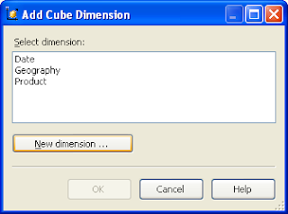
1. Click on Add Cube Dimension icon in Dimension Usage tab as shown below. It will open Add Cube Dimension dialogue box.

2. Click on New dimension… button in Add Cube Dimension dialogue box.

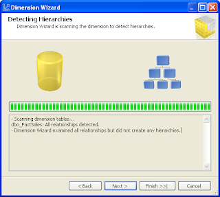
3. It will open Dimension Wizard. Click on Next to continue…
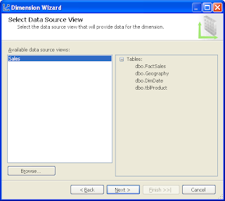
4. Select required data source view and click on Next to continue…

















5. Select Standard dimension option and click on Next to continue…
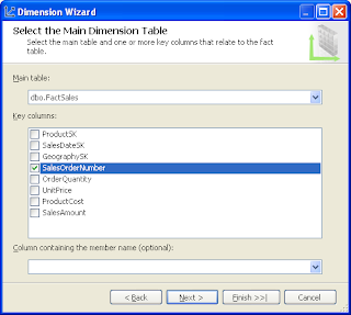
6. Select Main Dimension table and Key columns. Click on Next to continue…  

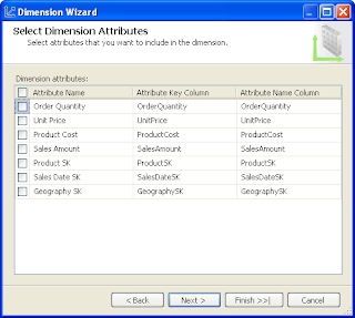
7. Select Dimension Attributes. Click on Next to continue…  

8. Click on Next to continue…  

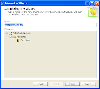
9. Now we are at Completing the Wizard. Give proper dimension name click Finish to complete.

 















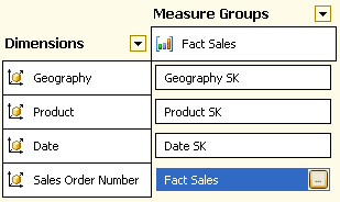
10. Newly created dimension is now available in Dimension Usage tab. At the intersection of Fact Sales measure group and the Sales Order Number dimension, click the ellipsis button (…) in the Item Description cell to review the fact relationship properties.   

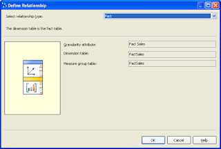
The Define Relationship dialog box opens. Notice that you cannot configure any of the properties. The Selected relationship type should be Fact.

The following image shows the fact relationship properties in the Define Relationship dialog box

Key Performance Indicators (KPIs) using Analysis Services

In business terminology, a KPI is a quantifiable measurement for gauging business success. In Analysis Services, a KPI is a collection of calculations that are associated with a measure group in a cube that are used to evaluate business success. Typically, these calculations are a combination of Multidimensional Expressions (MDX) expressions or calculated members. KPIs also have additional metadata that provides information about how client applications should display the results of the KPI's calculations

Common KPI Terms:

• Goal - An MDX numeric expression or a calculation that returns the target value of the KPI.
• Value - An MDX numeric expression that returns the actual value of the KPI.
• Status - An MDX expression that represents the state of the KPI at a specified point in time. The status MDX expression should return a normalized value between -1 and 1. Values equal to or less than -1 will be interpreted as "bad" or "low." A value of zero (0) is interpreted as "acceptable" or "medium." Values equal to or greater than 1 will be interpreted as "good" or "high."
• Trend - An MDX expression that evaluates the value of the KPI over time. The trend can be any time-based criterion that is useful in a specific business context. The trend MDX expression enables a business user to determine whether the KPI is improving over time or degrading over time.
• Status indicator - A visual element that provides a quick indication of the status for a KPI. 
• Trend indicator - A visual element that provides a quick indication of the trend for a KPI. 
• Display folder - The folder in which the KPI will appear when a user is browsing the cube.
• Parent KPI - A reference to an existing KPI that uses the value of the child KPI as part of computation of the parent KPI. Sometimes, a single KPI will be a computation that consists of the values for other KPIs.
• Weight - An MDX numeric expression that assigns a relative importance to a KPI. If the KPI is assigned to a parent KPI, the weight is used to proportionally adjust the results of the child KPI value when calculating the value of the parent KPI.

Creating KPIs using Business Intelligence Development Studio (BIDS)

1. Click on the KPIs tab
2. We shall first add a KPI named ProfitPercentage to the cube:
• Click on the New KPI button or right-click on the KPI Organizer window and select New KPI.
• In the KPI Designer which opens up, type in the name of the KPI as ProfitPercentage.
3. Add the measure to the Sales Fact measure group by selecting from the Associated measure group drop down.
4. Now let's add an expression to evaluate the value property of the KPI:
• Type the following expression in the Value Expression box. You could also drag the measures from the Metadata tab in the Calculation tools window.
  
  [Measures].[Profit]/[Measures].[Product Cost]
  OR
  ([Measures].[Sales Amount]/[Measures].[Product Cost]-1
  We have built the expression above using the logic that ProfitPercentage is calculated as the difference in Sales and Cost, divided by the Cost.
  Here [Measures].[Profit] is Calculated Member using below calculation:
  CREATE MEMBER CURRENTCUBE.[MEASURES].[Profit]
  
  
  AS SUM
  (
  [Date].[Calendar Year - Qtr - Month].currentmember,
  [Measures].[Sales Amount]-[Measures].[Product Cost]
  ),
  FORMAT_STRING = "#,#",
  VISIBLE = 1;
5. Now, let us set the goal of the KPI to a constant. Enter 0.25 in the Goal Expression box, which means the goal expects 25% more in sales than the cost.
6. Next we are on to the all important status. Here we shall write an expression to compare the value with the goal: 
• Before examining the actual expression let us take a look at a pseudo-expression:
  CASE
     WHEN value/goal >= 0.9 THEN 1
     WHEN value/goal < 0.8 THEN -1
     ELSE 0
  END
  
  Here, a ratio of .9 would be considered good in this instance. This means that if the value makes up at least 90% of the goal then it would be considered as successful, hence the value 1 to indicate it. If value/goal equals to less than 0.8 then the status will be considered as a failure (-1). And all those values do not fall into the above ranges will be considered neutral (0).
  
  Now, enter the following MDX expression into the Status expression box:
  CASE
     WHEN KPIValue("ProfitPercentage")/KPIGoal("ProfitPercentage")>=.9 THEN 1
     WHEN KPIValue("ProfitPercentage")/KPIGoal("ProfitPercentage")< .8 THEN -1
     ELSE 0
  END
  
  Being the realization of the previous "pseudo-expression", the above expression replaces value with KPIValue("ProfitPercentage") and goal with KPIGoal("ProfitPercentage"). The KPIValue function returns the value of the KPI's value property, while the KPIGoal function returns the value of the KPI's goal property. Both functions take the name of the KPI through a character string parameter.
7. Select an appropriate image type from the Status indicator drop down to provide for the visuals of the KPI status.
8. The next property to be configured is the trend. Once again, let us first look at a "pseudo-expression":
   CASE
      WHEN IsEmpty(x) THEN 0
      WHEN v - vX >= 0.25 THEN 1
      WHEN v - vX < -0.1 THEN -1
      ELSE 0
   END
   
   Here, x is the current time period of the previous year. For instance if the current selected time period is 20-May-2008, x will be 20-May-2007. v is the value of the KPI, which by default would return the value for the current time period. vx is the value of the KPI for the same time period of the previous year. The expression first checks if x is empty, thereby resulting in 0 (or no change in trend). Then, it checks if the current period's value is an increase of at least 25%, thereby indicating 1 or a positive trend. If there's a decrease of more than 10% from last year it indicates a negative trend or -1. All other results will indicate no change in the trend (or 0).
   
   Enter the following MDX expression in the Trend expression textbox:
   CASE
   WHEN IsEmpty(ParallelPeriod([Date].[Calendar Year - Qtr – Month].[Calendar Year], 1,[Date].[Calendar Year - Qtr – Month].CurrentMember)) THEN 0
   WHEN KPIValue("ProfitPercentage")-(KPIValue("ProfitPercentage"), ParallelPeriod([Date].[Calendar Year - Qtr - Month].[Calendar Year],1,[Date].[Calendar Year - Qtr - Month].CurrentMember)) >= 0.25
   THEN 1
   WHEN KPIValue("ProfitPercentage") - KPIValue("ProfitPercentage"),
   ParallelPeriod([Date].[Calendar Year - Qtr - Month].[Calendar
   Year],1,[Date].[Calendar Year - Qtr - Month].CurrentMember)) < -0.1 THEN -1
   ELSE 0
   END
   
   In the MDX expression above, x is replaced by ParallelPeriod([Date].[Calendar Year - Qtr - Month].[Calendar Year], 1,[Date].[Calendar Year - Qtr - Month].CurrentMember) ParallelPeriod is a function which returns a member from a prior period in the same relative position as a specified member. The variable v is replaced by KPIValue("ProfitPercentage") and vx is replaced by (KPIValue("ProfitPercentage"), ParallelPeriod([Date].[Calendar Year - Qtr - Month].[Calendar Year], 1,[Date].[Calendar Year - Qtr - Month].CurrentMember)).
9. Select an appropriate image type from the Trend indicator drop down to provide for the visual of the KPI trend. Here's a sample of what the KPI designer should look like:
   
   
   
10. 
    
    The KPIs is done! Next, process the cube. You will be able to view the KPIs using the built-in KPI Browser under the KPIs tab in BIDS. You could also use Office 2007 Excel.
    
    
    
    
    
     

Sort Dimension Members in DESCending order

Sometimes we need to display Date dimension members in descending order. For example, Client ask to show Calendar Year in DESC order.

But Analysis Services doesn't provide a way to sort dimension members in Descending order. SSAS provides only Ascending order.

However, we can achieve this sort functionality by using a simple trick. I will take an example to display Calendar Year member in DESC order. Below are the steps to achieve our goal:

Step1: Go to Data Source View (DSV) and right click on Date dimension in DSV diagram. Click on New Named Calculation... to create a new member.

Step2: Now enter CalendarYearSort in Column name and 0-CalendarYear in Expression textbox. This additional column will be used to sort calendar year in descending order. Click OK to proceed. Here I considered that CalendarYear is existing column in the dimension.

Step3: Go to Dimension Structure of Date dimension and drag and drop new member "CalendarYearSort" in attributes list.

Step4: Click on Attributes Relationship tab. Right click on Calendar Year member and select New Attribute Relationship... It will open Create Attribute Relationship wizard.

 

Step5: In Create Attribute Relationship, select Related Attribute as Calendar Year Sort and Relationship type as Rigid. Click OK to proceed.

Step6: Again go back to Dimension Structure tab and click on Calendar Year attribute. Go to properties and set following things as shown below:

OrderBy: AttributeKey and OrderByAttribute: CalendarYearSort

Step7: Now Calendar Year is set in decending order. Just save and process the cube.

Note: Before processing the cube, you can set AttributeHierarchyVisible = FALSE because we should not show this attribute in cube and AttributeHierarchyEnabled = False to reduce cube space and increase the performance.

Dynamic Cube Partitioning in SSAS 2008

In this article I am going to explain the Implementaion of Dynamic Cube Partition in SSAS 2008. I would want to split this article in two parts as mentioned below:

1. Partition benefits
2. Implementing Dynamic Partitions

Partition Benefits:

• Better Query Performance: Cube partition is a powerful mechanism for improving query performance. Queries that summarize data over 10 years could take considerably longer than those that only search through the current year data. If we have proper partitions then SSAS only has to scan a small subset of data to return query results hence dramatic performance improvements compared to queries running against a cube with a single partition.
• Minimize downtime:  Cube partitioning supports reducing downtime associated with cube processing. In almost all the cases, a portion of data warehouse is volatile and needs to be processed often. However other portions are relatively static. For example, in a sales cube, we need to change the current year's data nightly, but sales from previous years might change only occasionally - in case if account for merchandise returns and exchanges. If your warehouse tracks last 10 years salesthen processing only the current partition may be 10 times quicker than processing the entire cube.
• Aggregations benefits: The partition queried frequently could benefit from additional aggregations, which in turn could improve performance. Partition(s) that are used less can be processed less frequently with considerably fewer aggregations.
• Customized storage and processing settings: Frequently accessed partitions might benefit from proactive caching and ROLAP storage. On the other hand, other forms of storage and processing might be better for less frequently queried partitions.
• Distributed query and processing load: SSAS allows you to create remote partitions - a remote partition resides on a server different from its parent cube. This way the queries that affect the remote partition are processed on a server separate from its parent cube, allowing you to take advantage of additional processing power.
• Parallel Partitions Processing: SSAS allows processing multiple partitions in parallel on a server that has multiple processors. This can further reduce the total cube processing time.

 Implementing Dynamic Partitions

In this section I will explain step by step operations to create Dynamic Cube Partitions.

STEP1:
Preapare test data for Sales cube. I will use three dimensions (DimDate, DimProduct, and DimCustomer) and one fact table for Sales cube. Click here to download CubePartitionData.sql file which contains T-SQL code to generate these tables along with sample data.

STEP2:
Create new Analysis Services Project using BIDS and save it as Sales.

STEP3:
Create Data Source, and then Data Souce View using above three dimension tables.

If you are newbie, click Creating First Cube in SSAS 2008 for more information.

STEP4:
Create Sales cube  along with required dimensions. Set all  required properties of dimensions and create any hierarchies if required. My Solution looks like this:

STEP5:
Double click on the cube and navigate to Partition tab. You will see a default partition as shown below:

Delete this default partition and Click on new partition... to click new partition. In Partition Wizard, Select FactSales as available table in Specify Source Information page and click next. Select Specify a query to restict row in Restrict Rows page and write WHERE condition to restrict partition rows.

Click Next twice and enter Partition name Sales_20100101-20100131 in the Completing the Wizard page and click Finish.
Finally Process the cube. Once cube is processed successfully, you can see a new database in Analysis Services:

You can browse the data for this partition:

STEP6:
We are done with one manual partition. Now its time to create the partitions dynamically and apply a logic to process the delta data every time.

First off all, right click on the Partition Sales_20100101-20100131 (highlighted above)  and then select Script Partition as ==> Create To ==> New Query Editor Window. It will create XMLA scripts for this partition. Save this file in the project with CreatePartitionSales_20100101-20100131.xmla name.

In similar fashion, right click on the Partition Sales_20100101-20100131 and then select Process. This will open Process Partition wizard, click Script to generate XMLA script and save this file in the project with CreatePartitionSales_20100101-20100131.xmla name.

STEP7:

We are done with SSAS development! Now we have to create an SSIS package to implement dynamic creation of cube partition and processing of that partition.

Click on File => Add => New Project in menu bar in the same solution. Select Integration Services Project and enter the name of the SSIS Project.
Rename the SSIS package1.dtsx by DynamicSalesPartition.dtsx.

STEP8:
Add two connection Managers - one OLE DB connection manager for database and another Analysis Services connection manager for SSAS database.

STEP9:
Add following Package variables:

Here is the brief description of each variable:

Directory - To store package path
FromDateKey - To Store current partition start date key e.g. 20101201.
ToDateKey - To Store current partition end date e.g. 20101231
PartitionName - Current partition name e.g. SalesPartition_20101201-20101231
IsPartitionExists - To check whether partition alreday exists or not
CreatePartitionXMLA - To store XMLA script to create current partition
ProcessPartitionXMLA- To store XMLA script to process current partition

Note: You can add more variables as per need and business requirement.

STEP10

Now you have to develop SSIS package as shown below:



First Execute SQL Task is used to initialize FromDateKey, ToDateKey, and PartitionName for the current partition. Use below query in this Task:
DECLARE
   @FromDateKey varchar(8), @ToDateKey varchar(8),
   @CalendarYear int, @CalendarMonth int


SELECT
   @FromDateKey = MAX(FromDateKey),
   @ToDateKey = MAX(ToDateKey)
FROM PartitionLog (NOLOCK)


SELECT
   @CalendarYear = MIN(CalendarYear),
   @CalendarMonth = MIN(CalendarMonth)
FROM DimDate WHERE DateKey > @ToDateKey + 1


--SET FromDateKey and ToDateKey for current Partition
IF NOT CONVERT(varchar(8),GETDATE(),112) BETWEEN @FromDateKey AND @ToDateKey
SELECT @FromDateKey = MIN(DateKey), @ToDateKey = MAX(DateKey)
FROM DimDate (NOLOCK)
WHERE CalendarYear = @CalendarYear AND CalendarMonth = @CalendarMonth


SELECT @FromDateKey AS FromDateKey, @ToDateKey AS ToDateKey,
'Sales_' + @FromDateKey + '-' + @ToDateKey AS PartitionName
GO

Second Task in the package is Script Task. Here we need to read the contents of files
CreatePartitionSales_20100101-20100131.xmla and
ProcessPartitionSales_20100101-20100131.xmla and store in the package variables CreatePartitionXMLA & ProcessPartitionXMLA.

I am using User::Directory as ReadOnlyVariable and User::CreatePartitionXMLA,User::ProcessPartitionXMLA as ReadWriteVariables.


Click here to download the code for Script Task - Read XMLA Files and store in variables.

To know about reading file contents using Script Task, click Script Task to Read File.

Third Task is a sequence container which contains three task - Script Task, Analysis Services Execute DDL Task, and Execute SQL Task.

Script Task is used for two reasons -
1. To check whether current partition exists or not.
2. To update XMLA content for current Partition.

This is the most tricky and interseting part here. We need to replace Partition ID, Partition Name, and Source QueryDefinition for current Partition which are highlighted below:

In Script Task, select User::FromDateKey,User::PartitionName,User::ToDateKey as ReadOnlyVariables and User::CreatePartitionXMLA,User::ProcessPartitionXMLA,User::IsPartitionExists as ReadWriteVariables.

Click here to download the code for Script Task - Generate XMLA to create and Process new Partition.

Click SSIS Script Task to Find and Replace File contents to know more about find and replace mechanism using script task.

Second task in the sequence Container is Analysis Services Execute DDL Task. This task is used to create new Partition. In Analysis Services Execute DDL Task Editor, select SSAS.localhost as Connection, Variable as SourceType, and User::CreatePartitionXMLA as Source.

Also don't forget to set precedence constraint. You should execute this task only when partition does not exists. Open Precedence Constraint Editor and Select Expression and Constraint in Evolution operation, Success in Value, and @IsPartitionExists == 0 in Expression as shown below:

Third Task in the Sequence Container is Execute SQL Task - this is used to store newly created Partition information in the PartitionLog table. In Execute SQL Task, select ResultSet None, ConnectionType OLE DB, Connection (local).Test, SQLSourceType Direct input and SQLStatement as:

INSERT INTO dbo.PartitionLog
([PartitionName],[FromDateKey],[ToDateKey],[CreatedDate])
VALUES (?,?,?,GETDATE())

Click on Parameter Mapping and map the parameters as shown below:

STEP11
Finally we need to process the current partition. This is independent of previous sequence container where we are creating new partition if it is not exists.
However, we need to process the current partition every time we execute the package. In most of the cases, new partition will be created on the first day of month but partition should be processed everyday to include delta data.

This sequence container also contains three tasks.

First task is Analysis Services Processing Task - to process the dimensions data. Select SSAS.localhost as connection manager and all the dimensions in Object Name - which are not static in data. Select Process Update as Process Option.

Second Task is againg Analysis Serives Processing Task - to process Current Partition. Select SSAS.localhost as connection manager and Sales_20100101-20100131 in Object Name - which is default partition (or first partition). Select Process Full as Process Option.

Now click on Expression and select @[User::ProcessPartitionXMLA] in ProcessingCommands.

Finally store the Last Processed Date and Processed Count (number of time this partition has processed) in the log table using Execute SQL task. Select ResultSet None, ConnectionType OLE DB, Connection (local).Test, SQLSourceType Direct input and SQLStatement as:

UPDATE PartitionLog
SET LastProcessDate = GETDATE()
,ProcessedCount = ProcessedCount + 1
WHERE PartitionName = ?
 
Click on Parameter Mapping and map the parameters and map the parameter 0 with User::PartitionName.

STEP12
We are done with package development. Now its time to execute the package and check the dynamic behaviour of Partition creation and processing. Before execution the package, there is only partition in the SSAS Sale database.
Now Right Click on the package and execute it. Once package is execute successfully, you will see one more partition in the Sales database and one more entry in PartitionLog table.

 

Now Execute the package or schedule it to execute automatically. Once you are done with 10 more executions, you will reach to current month partition Sales_20101201-20101231. and you can see 12 partitions - one partition for each month as shown below:

Since you are in current month partition, if you execute the package every day in current month - it will not create any new partition till beginning of next month. It will only process Current Partition to include the data in the cube as shown below:

Now you can browse the data for all the partitions:

We are done with Dynamic Package creation.
I hope you will like this article and if your answer is yes then don't forget to click Like :-)

Many people have had asked me to share the solution. I have stored that in my SkyDrive so you can download it from here: Dynamic Cube Partition

Cheers!!!

 

Creating First Cube in SSAS 2008

Nowadays, analytical solutions are becoming mission critical for many organizations. Microsoft SQL Server 2008 Analysis Services (SSAS) is designed to provide exceptional performance and scalable support with millions of records and thousands of users from different locations.

Why to Build a Cube?
There are many advantages of cube over relational data mart.

• While querying a data mart, you can get most of the results but not everything you need for business analysis and decsion making. Cube can help you to get answers of all "What-If" scenarios.
• Building a cube helps to house your data to centralize the business rules for calculations that you can't easily store in a relational data mart.
• The structure of the cube makes it much easier to write queries to compare data year over year (YOY), or to create cumulative values such as year-to-date (YTD) sales.
• Scalable Infrastructure - Analysis Services can scale to support databases of many terabytes in size with many thousands of users.
• Superior Performance - Analysis Services cubes are multidimensional structures that enable fast access to high volumes of pre-aggregated data, empowering end users to gain insight into relevant business data at the speed of thought.
• You gain the ability to manage aggregated data in the cube. To improve query performance in a relational data mart, we often create summary tables to prepare data for queries that don't require transaction-level detail. SSAS creates the logical equivalent of summary tables (called aggregations) and keeps them up-to-date.

I would like to introduce beginners to Microsoft SQL Server Analysis Services (SSAS) by creating a simple cube from AdventureWorksDW2008R2. You can install this database from codeplex.

I'll cover following things in this article:

1. Creating Analysis Services Project
2. Creating Data Source
3. Creating Data Source View
4. Creating Cube and Dimensions
5. Creating Dimension Hierarchies
6. Deploying Cube Database from BIDS

Creating Analysis Services Project.

First step is to create a project in Business Intelligence Development Studio (BIDS). Launch BIDS from Start --> All Programs --> Microsoft SQL Server 2008 --> SQL Server Business Intelligence Development Studio and then click File --> New --> Project. In the New Project dialog box, select Analysis Services Project. In the Name text box, type LearnSSAS and, if you like, change the location for your project. I'll store this project at location D:\Hari. Click OK to create the project.

 

Creating Data Source

Now add a data source to define the connection string for data mart AdventureWorksDW2008R2. In Solution Explorer, right-click the Data Sources folder and click New Data Source.

In the Data Source Wizard, click Next on the Welcome to the Data Source Wizard page if it hasn't been disabled. On the Select how to define the connection page, click New to set up a new connection. In the Connection Manager, the default provider is the Native OLE DB\SQL Server Native Client 10.0, which is correct for our project.

To define the connection, type the name of your server in the Server Name text box. Alternatively you can select it from the drop-down list, then select AdventureWorksDW2008R2 in the database drop-down list and click Test Connection button to check the connection. Finally click on OK as shown below:

 

When you're back in the Data Source Wizard, click Next. On the Impersonation Information page, select Use the service account option so that service account will be used to read data from the source when loading data into your SSAS database and service account  must have read permissions to do so. Click Next and then Finish to complete the wizard.

 

Creating Data Source View

Now next step is to create a data source view (DSV) from the data source to define dimensions and cubes. You can make changes to the DSV without modifying the actual data source, which is very useful if you have only read permissions to the data mart. In Solution Explorer, right-click on the Data Source Views folder and then click New Data Source Views...You can see Data Source View Wizard. Click Next on the Welcome page. On the Select a Data Source page, select the data source just added to the project (Adventure Works DW2008R2.ds) and click Next. Now add required objects to the DSV by double-clicking each table or view on Select Tables and Views page. I want to add the following tables to the DSV to make it easy to understand for beginners:

DimDate, DimProduct, DimProductCategory, DimProductSubcategory, and FactInternetSales. You can always add more tables later if you want to explore advance BI questions. Now click Next in the Data Source View Wizard once you are finished adding required tables followed by click on Finish. You can give a name to your DSV before clicking Finish button.

I would recommend you to change the name of objects by selecting each one in the DSV designer and remove the Dim and Fact prefixes from the FriendlyName property because when you create dimensions and cubes, only FriendlyName property will be assigned to the objects.

The DSV is shown below:

 

Creating Cube and Dimensions

Next step is to create a Cube and Dimensions from the data source view. In Solution Explorer, right-click on the Cubes folder and then click New Cube...You can see Cube Wizard. Click on Next in Welcome to the Cube Wizard page.On the Select Creation Method page, keep the default option Use existing tables and click Next button. On the Select Measure Group Tables page, choose InternetSales table and click Next.

Now the wizard displays all the measures available in the selected measure group tables. Measures are basically numeric values e.g. OrderQuantity, Unit Price, Sales Amount, Tax Amount etc. Select only the following measures from Internet Sales Group: Order Quantity, Unit Price, Total Product Cost, Sales Amount, and Internet Sales Count

Now click on Next button to open Select New Dimensions page and select Date and Product dimensions. Click Next to proceed.

In the Completing the Wizard page, enter the cube name as AdventureWorksCube and click Finish button to complete the wizard. Cube layout is shown below:

Now click on each dimensions and add required attributes from the Data Source View.

Date Dimension:

Drag and drop FullDateAlternateKey, CalendarYear, CalendarQuarter, EnglishMonthName, and EnglishDayNameOfWeek. Rename FullDateAlternateKey with Full Date, EnglishMonthName with Calendar Month, and EnglishDayNameOfWeek with Calendar Week as shown below:

Product Dimension:

Drag and drop EnglishProductCategoryName from ProductCategory table, EnglishProductSubcategoryName from ProductSubcategory table and Color, ModelName, Size and Weight from Product table.

Creating Dimension Hierarchies

Navigate to Date Dimension Structure. Drag and drop Calendar Year attribute into Hierarchies surface area following by Calendar Quarter, Calendar Month, Calendar Week , and Full Date attributes.

Rename hierarchy with Calendar. You'll see a warning mark in the hierarchy because attribute relationship is not set properly.

Set Attribute Relationships

Click on the Attribute Relationships tab in the dimension designer. This tab is available only in Analysis Services 2008. By default, all attributes relate directly to the key attribute, Date Key as shown below:

To optimize the design by reassigning relationships, Right Click on Full Date and select New Attribute Relationship. Select Related Attribute as Calendar Week and Relationship type as Rigid (will not change over time). Repeat same thing for remaining attributes. Finally Attribute Relation will look like below image:

Deploying Cube Database from BIDS

Now its time to deploy the cube at required server. Right click on the project (LearnSSAS in this example) and click properties to open project properties page. Enter Server Name name Server property and Database name in Database property as shown below:

Click OK to save changes. Now right click on the project and click on Process to Build and Deploy the project. You will a message while deploying the database first time.

Click on Yes to proceed. Now you can see Process Database - PreojectName window. Click on Run to continue.

Once the database is deployed and processed successfully, you can see the data through Browser tab or directly through SQL Server Analysis Services. You can also pull cube data in Excel using Excel OLAP Pivot Tables, which is the prefered option used by business managers.